Manual

Second Moment Data Analysis:

The second momdent analysis will calculate weight-average sedimentation coefficients for each scan included in the analysis by finding the second moment point in the boundary. The second moment analysis can serve as a valuable diagnostics tool in identifying problems such as time-dependent degradation, aggregation and even concentration dependency. It is important to keep in mind that the second moment analysis is only valid for scans that have cleared the meniscus and still have a stable plateau. All other scans should be excluded from the analysis.

You start the Second Moment data analysis by clicking on "Second Moment" in the Velocity sub-menu of the main menu. The main Second Moment data analysis window will appear.

The first step in the analysis requires that you load an UltraScan dataset that has previously been edited with the UltraScan editing module. UltraScan sedimentation velocity datasets always have the suffix ".us.v". Click on the "Load Dataset" button in the left upper corner of the control panel. Simply select the desired run from the selection of available runs in the dataset loading dialog. Once loaded, the Run Details will be shown. Click on the "Accept" or "Cancel" button, and you will be returned to the analysis window, which will show the first available dataset of the selected run in the edited data window on the lower right panel, and the Second Moment analysis will be shown in the upper right panel of the analysis window.

Analysis Functions:

Click on these buttons to control the Second Moment analysis: Load Data: Load edited data sets (with the *.us suffix). A file dialogue will allow you to select a previously edited and saved velocity experiment. If the data was edited with an older version of UltraScan than the current, an error message will be displayed. Run Details: View the diagnostic details for a particular run. Reset Data - use this button to reset the default settings for the analysis. Save Data: Write out a copy of all results to an ASCII formatted data file suitable for import into a spreadsheet plotting program. See "File Structures and Formats" for details. Note: These files are overwritten each time this button is clicked. Only the last version of the analysis will be saved! Print Data: Load the printer control panel for printing of plot graphics View Data Report: See the data report for the last analysis setting. Note: This file is re-written each time it is accessed. Only the current analysis result is available. Help: This help file Close: Close the Second Moment analysis window.

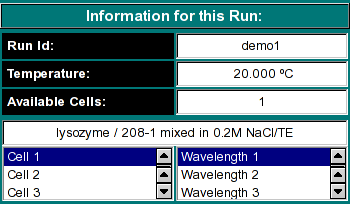
Run Information:

Run ID: The name of the run given during editing Temperature: The average temperature calculated from the entire run Available Cells: The numbers the cells that contain analyzable data Clicking on a cell and wavelength selection will bring up the cell contents description for that cell and wavelength. Scroll through this list to bring up information for cells > 3. If there is no data available for the selected cell, the program will list "No Data available". Selecting a cell/wavelength combination will automatically bring up the corresponding dataset and present the analysis.

Experimental Parameters:

Here you can enter the corrections for density, viscosity, and partial specific volume of your sample. As you change the information in these fields, the program will automatically update the analysis to correct the S-value according to the specified buffer conditions. If the data was retrieved from the database and associated with the correct buffer file and peptide file, the density, viscosity and partial specific volume (vbar) will automatically be updated to the appropriate values and don't need to be adjusted to produce S 20,W corrected values. Density: Click to calculate the density based on the composition of your buffer. Viscosity: Click to calculate the viscosity based on the composition of your buffer. vbar(20o): Click to calculate the partial specific volume for a peptide based on its primary amino acid sequence and correct the vbar value for the current temperature. Skipped: This field refers to the scans at the beginning of the run that are excluded from the analysis. the van Holde - Weischet analysis requires that the scans have cleared the meniscus in order to be analysable. If they haven't cleared the meniscus, they are automatically excluded from the analysis. Note: This number may change if the percentage and position of the analyzed boundary are changed (see below).

Analysis Controls:

Data Smoothing: Use this feature to smooth the experimental data. For noisy data, increasing this parameter can improve the clarity and appearance of the results considerably. Please note: Whenever possible, especially for very steep boundaries with low diffusion, try to avoid using too much smoothing to prevent artificial modification of the boundary shape. Smoothing is performed based on a frame average. The number shown represents the size of the smoothing kernel used (the number of datapoints averaged for a single point). The algorithm used is non-destructive of the original data and hence the smoothing is reversible. Also, point smoothing is independent, where the smoothing of one point does not have any effect on the smoothing of its neighbors. Only unsmoothened points are used for the calculation of the smoothed value. Each time you click on the counter, the current dataset will be reset to the full dataset. % of Boundary: This is the portion of the boundary used for the analysis. 100 % refers to the entire boundary, reaching from the baseline concentration value to the plateau concentration value. This portion is shown in yellow in the experimental data plot at the lower right panel of the van Holde - Weischet analysis window. Excluded data is shown in blue. Changing this number will automatically reset the position of the analyzable portion of the boundary in the center of concentration between the baseline and the plateau concentration. Boundary Position (%): For percent-boundary values less than 100 %, this number refers to the percentage of total concentration by which the remainder (=un-analyzed portion of the boundary) is shifted away from the baseline. A value of 0% refers to a data analysis start at the baseline. This number is always less than or equal to 100 % - (% of Boundary). It allows you to control the position of the analyzed portion relative to the baseline. The blue colored portion of a scan is excluded from the analysis, and the yellow portion is analyzed. Exlude Single Scan: When setting this counter to a non-zero value, the respective scan will be highlighted in red. Clicking on "Excl. Single Scan" while a scan is highlighted in red will delete this scan from the analysis. Deleting scans from the analysis is irreversible and can only be reset by clicking on the "Reset" button or by reloading the data (when smoothing, the data is always automatically reloaded, causing the number of scans to be reset to the original count). Skipped scans are excluded automatically, because they haven't cleared the meniscus. This is equivalent to scans whose first point has an absorbance larger than the baseline (as defined by the baseline absorbance selected during editing). Second moment points for these scans will be displayed in red and excluded from the average, which is displayed as a horizontal line in the second moment plot. Exclude Scan Range: Same as "Exclude Single Scan", except for multiple scans. To use this feature, select first the start scan of the range by using "Exclude Single Scan", then complete the scan range by using "Exclude Scan Range". Just like the van Holde - Weischet analysis, the Second Moment analysis also requires that scans have cleared the meniscus and contain a stable plateau in order to be valid scans for inclusion in the analysis. Please see the van Holde - Weischet analysis tutorial to decide which scans are appropriate for analysis and which scans need to be excluded. Status: The status bar informs the user about the progress of the analysis. On slower computers this has more significance than on a fast Unix machine.

Utility of Second Moment Analysis:

The Second Moment Analysis provides useful diagnostics to determine certain properties of a velocity experiment. It will not, however, provide information about the distribution of S-values present in the sample. The van Holde - Weischet methods is better suited for this purpose. The strength of this method is its ability to detect the following features:

• Concentration dependent non-ideality - A concentration dependent sample starts out with a low second moment S-value and increases as the concentration drops due to radial dilution. Eventually, it will plateau at the true second moment S-value.
• Concentration dependent self-association - If you are looking at a self-associating system, such as a monomer-dimer equilibrium, the radial dilution will shift the average S-value towards the monomer when radial dilution reduces the concentration. This will most likely reduce the average S-value over the course of the run.
• Sample Degradation - A degrading sample will have a continuous decrease of the second moment S-value throughout the run
• Sample Pelleting - A sample exhibiting pelleting (loss of absorbance) will also reduce the second moment S-value over time. The difference between this condition and sample degradation is that pelleting samples will generally not show a reduced second moment S-value until the later scans are reached.
• Aggregation - A sample which aggregates over time, the second moment S-values will increase towards the end of the run, with no plateau forming.