Manual

Combining Molecular Weight distributions:

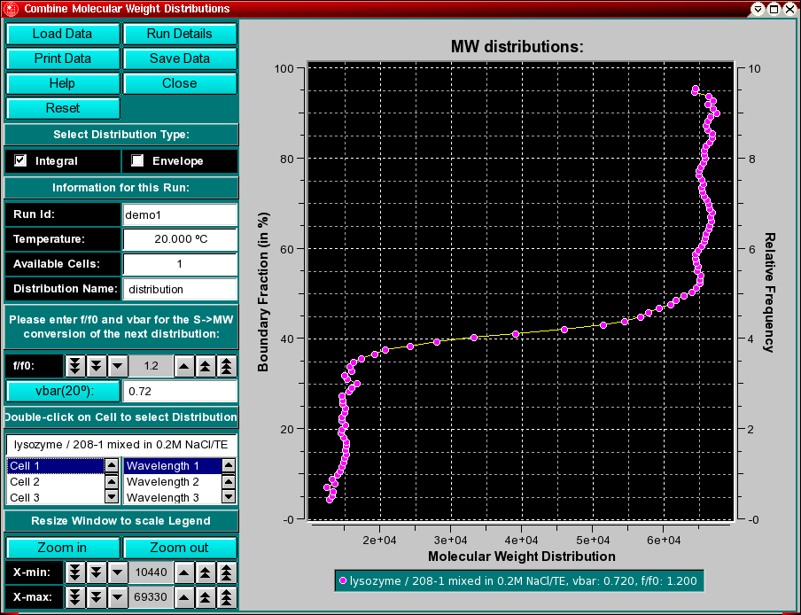
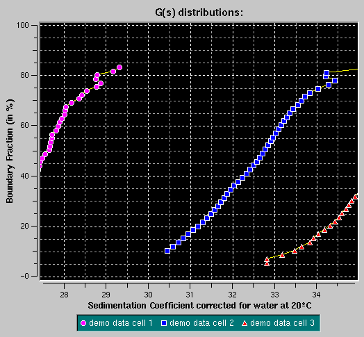
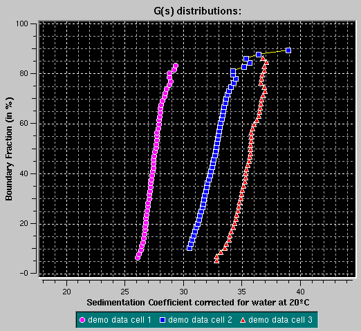
This program enables you to convert integral van Holde - Weischet G(s) distributions from S,20W values to molecular weight distributions for a given partial specific volume and an estimate for the f/f0 value. To combine multiple datasets (either from different cells of the same run or from different runs), use the "Combine Molecular Weight Distributions" item from the Utilities menu. This will allow you to compare molecular weight distributions (which are derived from integral distributions) from different runs and different cells to each other. This may be useful if you analyzed the same sample under different conditions, for example, different pH levels or different concentrations. If the samples are the same, the distributions should overlay, if the samples behave differently, the distributions will be shifted against each other.

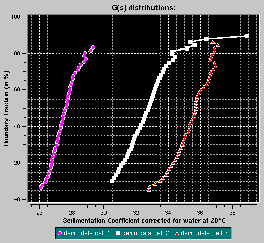
All distributions will be plotted relative to the boundary fraction they were analyzed. For example, if you analyzed 100% of the boundary, the distribution will range from 0 % - 100 % of the Y-axis. A distribution that was analyzed from 72 % of the boundary, shifted 8 % from the bottom will be plotted from 8 % to 80 % of the Y-axis. It is important that this distinction be made, since, for example, concentration dependent samples will behave differently depending on the position in the boundary, or heterogeneous samples will show different distributions depending which portion of the boundary was analyzed.

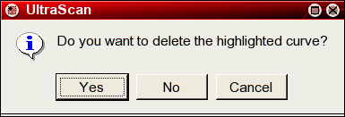
You can remove erroneously added distributions by double clicking on the distribution to remove it. The curve will be highlighted in white and a message window will ask you if you want to delete it. Confirm or cancel.

Explanation for fields and buttons:

Click on these buttons to control the van Holde - Weischet analysis. Load Data: Load edited data sets (with the *.us suffix). A file dialogue will allow you to select a previously edited and saved velocity experiment. If the data was edited with a version of UltraScan less than the current version, an error message will be displayed. Run Details: View the diagnostic details for a particular run. Print Data: Load the printer control panel for printing of plot graphics Save Data: Write out a copy of all distributiones to an ASCII formatted data file suitable for import into a spreadsheet plotting program. The data will be saved in a file called "mw_distrib.dat" in your results directory (see configuration panel). See "File Structures and Formats" for details. The descriptions in the legend for each dataset is saved in an ASCII file called "mw_distrib.txt". Note: These files are overwritten each time this button is clicked. Only the last version of the analysis will be saved! Help: This help file Close: Close the "Combine G(s) Distribution" window. Reset: Reset the plot window and delete all distributions and the legend. After clicking on "Reset" you can start with a new, empty plot window.

Run Information:

Run ID: The name of the run given during editing Temperature: The average temperature calculated from the entire run Available Cells: The numbers the cells that contain analyzable data Distribution Name: The name under which the html report will be saved. If you make this name the same as the dataset, the combined distribution data will be included in the html report for that dataset. If the default name "distribution" is left unchanged, a separate directory called "distribution" will be created under the html report directory. For more information on the html reports, please see the html report manual page.

Conversion Parameters:

f/f0: Use the counter to set an estimate for the f/f0 value. 1.0 corresponds to a spherical molecule. The larger the value, the more non-globular the molecule will be. An accurate f/f0 value needs to be entered if tbe molecular weight distribution is to be trusted. You have to include any hydration of the molecule in this value. vbar(20o): Click to calculate the partial specific volume for a peptide based on its primary amino acid sequence and correct the vbar value for the current temperature.

Plot Distribution Selection:

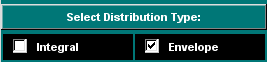Select the distribution type to be displayed in the plot. You can overlay different types of plots (integral distribution or histogram envelope or both) or overlay different distributions. When you click on the checkboxes, the next distribution to be added will be displayed in the format identified by the selected checkbox. The default setting is the integral van Holde - Weischet distribution.

Experimental Parameters:

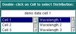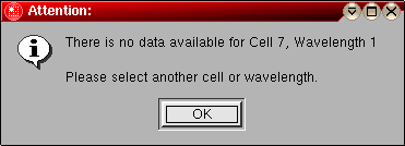
Single-clicking on a cell or wavelength will bring up the sample description of that cell and wavelength. If no data is available for your selection, it will be indicated in the top field. Double-clicking on a valid selection will add the integral distribution of that selection to the plot area and add an item to the legend. Scroll through this list to bring up information for cells > 3. 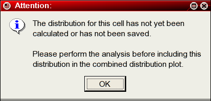If you double-click on an invalid item, an error message window will appear. If the selection is valid, but a distribution plot has not been saved from the van Holde - Weischet analysis, an error message will appear. If you decide to eliminate a distribution plot from the combined overlay, simply click on the scan to be removed in the plot area, and you will be asked if you want to delete the highlighted scan. The scan about to be deleted will be highlighted in white.

Analysis Controls:

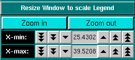Sometimes the legend does not appear correctly resized (for example, if the item in the description of the sample is too long for the provided screen area), In that case, it is necessary to resize the window to a larger size to accommodate the longer text. Click on "Zoom in" or "Zoom out" to present a smaller or larger scale of the item. Clicking on the X-min and X-max counters allows you to manually set the X-min/max limits of the data plot.