Manual

C(s)Analysis:

The C(s) analysis [P. Schuck (2000) Size distribution analysis of macromolecules by sedimentation velocity ultracentrifugation and Lamm equation modeling. Biophysical Journal 78:1606-1619.] can be used to generate sedimentation coefficient distributions from sedimentation velocity experiments. The principle of the method is based on finding non-zero terms in a linear combination of Lamm equation solutions describing the individual components in a sample. The coefficients of each term determine the partial concentration of each component. The method requires input of an upper and lower s-value boundary, an f/f0 frictional ratio, and a sedimentation coefficient resolution setting that determines the granularity of the linear combination. The frictional ratio is used to calculate a corresponding diffusion coefficient for each s-value term in the linear combination.

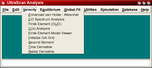
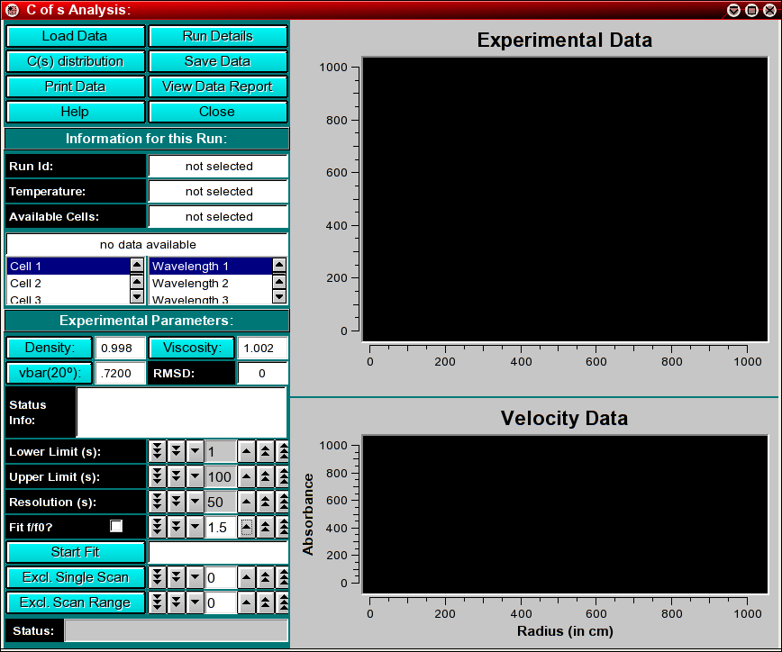
The C(s) analysis can be started in one of two ways: First, you can launch the application by clicking on "C(s) Analysis" in the Velocity sub-menu of the main menu. The main C(s) analysis window will appear. The second way to launch this application is from within the enhanced van Holde - Weischet Analysis. By using the van Holde - Weischet analysis, a model independent approach, a limit for the possible s-values present in the sample under investigation can be established before the C(s) analysis is performed. This eliminates the uncertainty introduced when the user selects these limits without prior knowledge, and it is therefore the preferred method to select the limits and to launch the application.

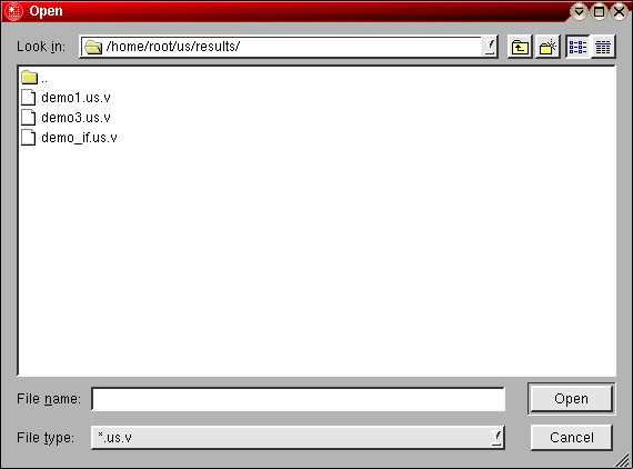
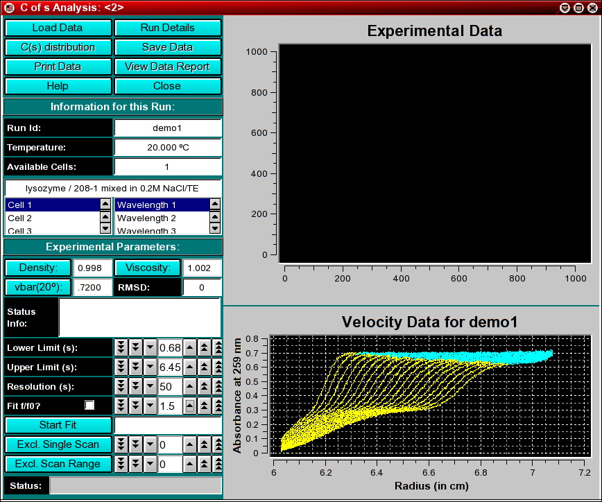
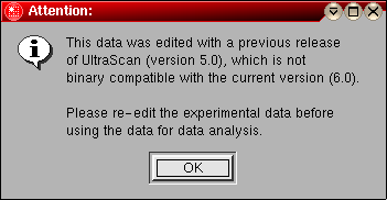
The first step in the analysis requires that you load an UltraScan dataset that has previously been edited with the UltraScan editing module. UltraScan sedimentation velocity datasets always have the suffix ".us.v". Click on the "Load Dataset" button in the left upper corner of the control panel. Simply select the desired run from the selection of available runs in the dataset loading dialog. Once loaded, the Run Details will be shown. Click on the "Accept" or "Cancel" button, and you will be returned to the analysis window, which will show the first available dataset of the selected run in the edited data window on the lower right panel.

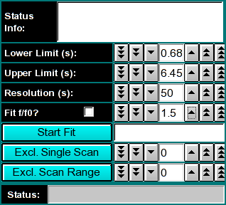
Next, confirm the upper and lower limits for the s-value distribution range to be fitted to your data. If you launched the application from the enhanced van Holde - Weischet analysis, these values will already be set to a suggested value, otherwise, a default range between 1s - 100s will be shown (which will not be appropriate for most applications). Also, a resolution setting needs to be selected. 20-50 is an appropriate default for the first analysis. This can be refined in subsequent iterations. Finally, an f/f0 value has to be selected. An f/f0 value of 1 corresponds to a molecule with a perfectly spherical shape, the larger the value is, the more non-globular the simulated shape will be. If you are not sure of the appropriate value for f/f0, leave it at the default value of 1.5.

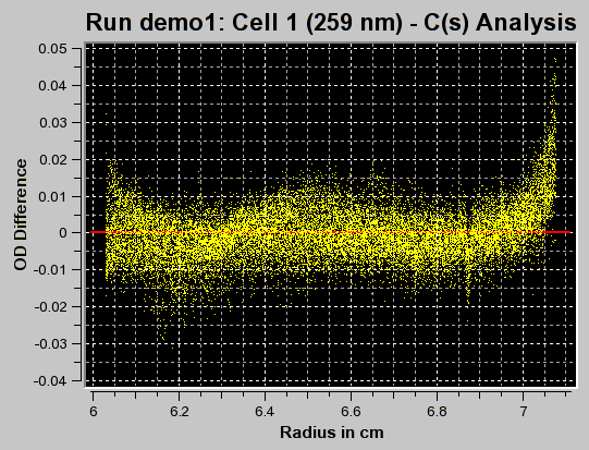
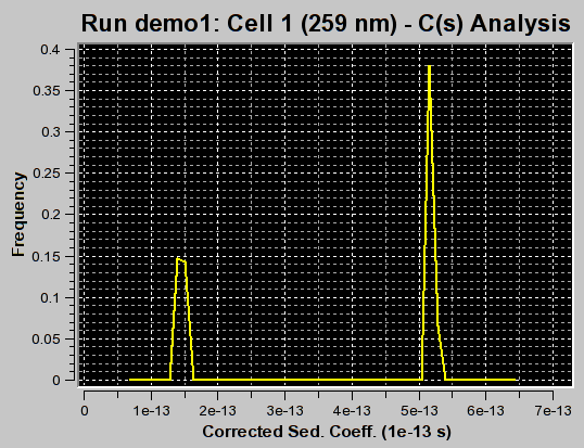
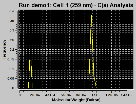
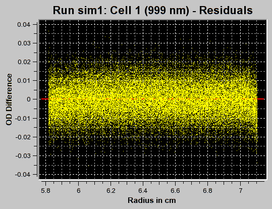
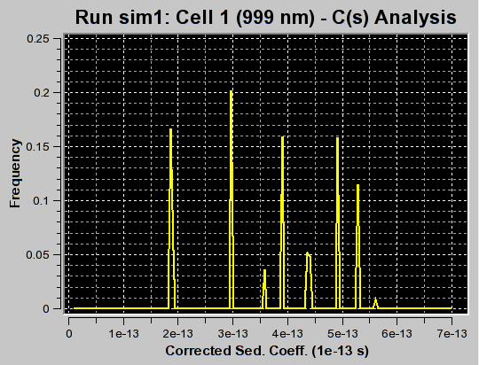
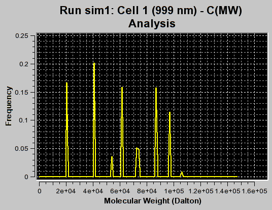
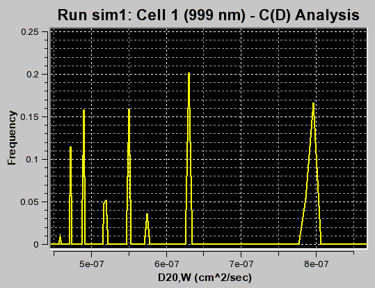
The first iteration should be made with the "Fit f/f0?" value left unchecked by clicking on the "Start Fit" button. A single iteration will be fitted (which will be fast) and provide an initial view of the s-value distribution appropriate for the sample. During fitting, the "Start Fit" button will change text to "Stop Fit". Clicking on it at any time during the fit allows you to abort a currently active fit. After the iteration is completed, the upper plot panel will show now the residuals of the fit. A red/green residuals pixels map is also shown in a separate window. Please refer to this link for more information on the residuals pixel map. The C(s)distribution can now be shown by clicking on the "C(s) Distribution" button in the upper left control panel. Once clicked on, the button will change text to show "MW Distribution". Clicking again, the fitted f/f0 value will be used to transform the C(s) distribution into a molecular weight distribution. At this point the button will change text again to show "Residuals". Repeatedly clicking this button will cycle through these three options.

Continue to adjust the upper and lower limits until an acceptable range of s-values has been determined by performing single fits. Generally, such a range is found when the spacing of peaks is well distributed throughout the range and no end effects are visible (large amplitudes at the end points of the distribution).

At this point one can fit for the most representative f/f0 value by selecting the f/f0 fitting checkbox. Clicking on the "Start Fit" button will then start a fitting session that tries to determine the optimal f/f0 value.

Important Note: The C(s) analysis can produce misleading results and artifactual peaks under certain conditions. If the f/f0 ratio is overestimated, additional artifactual peaks can occur.

Example:

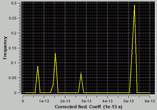
	f/f0=1.2 (appropriate for first peak and corresponding to the true C(s) distribution as verfified by van Holde - Weischet and finite element analysis)
	f/f0=3.1 (appropriate for second peak)
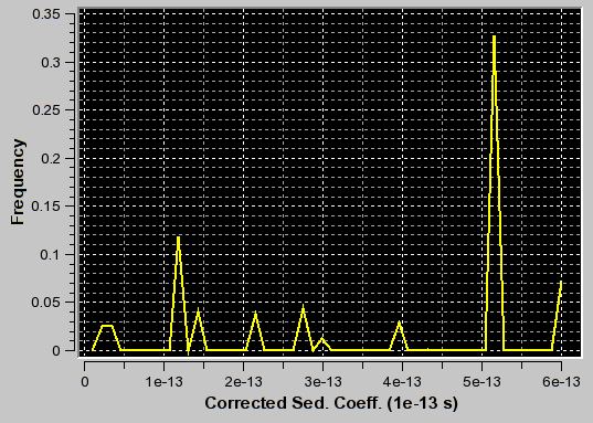	f/f0=3.1 (appropriate for second peak)

Please note this CAVEAT: For multi-component systems it is often unlikely that all species in the system have the same shape and hence the same f/f0 value. Therefore the molecular weight distributions will often be skewed and not necessarily represent the true molecular weights in the system. The f/f0 value determined by this method is only a best compromise between all possible f/f0 values.

Analysis Functions:

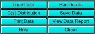Click on these buttons to control the enhanced van Holde - Weischet analysis. Load Data: Load edited data sets (with the *.us suffix). A file dialogue will allow you to select a previously edited and saved velocity experiment. If the data was edited with an older version of UltraScan than the current, an error message will be displayed. Run Details: View the diagnostic details for a particular run. C(s) Distribution: This button is a multi-function button that allows you to cycle through four different representations of the data analysis. All representations are shown in the analysis plot section of the module. The first representation is the residuals pattern, which is shown by default. To change the representation, click on the "C(s) Distribution" button to see the C(s) Distribution. After clicking, you will notice that the button has obtained a different label ("C(MW) Distribution"). The next time you click on it, the program will show the Molecular Weight Distribution obtained after transforming the C(s) distribution to a molecular weight distribution based on the f/f0 and vbar values shown in the Experimental Parameter section. The last representation is the C(D) Distribution, which will show the s-value transformation to a diffusion coefficient distribution based on the f/f0 and vbar values. Please note that the molecular weight and diffusion coefficient distributions are subject to the caveats discussed above ( caveat 1 and caveat 2). Save Data: Write out a copy of all results to an ASCII formatted data file suitable for import into a spreadsheet plotting program. Also save the plot images for a report. Note: These files are overwritten each time this button is clicked. Only the last version of the analysis will be saved! Print Data: Load the printer control panel for printing of plot graphics View Data Report: See the data report for the last analysis setting. Note: This file is re-written each time it is accessed. Only the current analysis result is available. Help: This help file Close: Close the van Holde - Weischet analysis window.

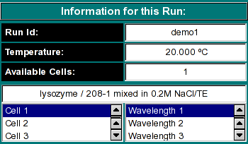
Run Information:

Run ID: The name of the run given during editing Temperature: The average temperature calculated from the entire run Available Cells: The numbers the cells that contain analyzable data Clicking on a cell and wavelength selection will bring up the cell contents description for that cell and wavelength. Scroll through this list to bring up information for cells > 3. If there is no data available for the selected cell, the program will list "No Data available". Selecting a cell/wavelength combination will automatically bring up the corresponding dataset and present the analysis.

Experimental Parameters:

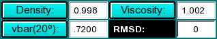Here you can enter the corrections for density, viscosity, and partial specific volume of your sample. As you change the information in these fields, the program will automatically update the analysis to correct the S-value according to the specified buffer conditions. If the data was retrieved from the database and associated with the correct buffer file and peptide file, the density, viscosity and partial specific volume (vbar) will automatically be updated to the appropriate values and don't need to be adjusted to produce S 20,W corrected values. Density: Click to calculate the density based on the composition of your buffer. Viscosity: Click to calculate the viscosity based on the composition of your buffer. vbar(20o): Click to calculate the partial specific volume for a peptide based on its primary amino acid sequence and correct the vbar value for the current temperature. RMSD: This field reports the residual mean square deviation from the fit. A value of < 0.007 is desirable for a good fit from absorbance data.

Analysis Controls:

Status Info: This widget provides information about the progress of the fitting process. Lower Limit (s): This field indicates the lower bound of the s-value distribution. Clicking on one of the arrow keys permits changing of the value in steps of 0.1 (one arrow), 1.0 (2 arrows) or 10 (3 arrows). Upper Limit (s): This field indicates the upper bound of the s-value distribution. Clicking on one of the arrow keys permits changing of the value in steps of 1.0 (one arrow), 10.0 (2 arrows) or 100.0 (3 arrows). Resolution (s): Select the number of basis functions in the linear combination of Lamm equations used to model the sedimentation distribution. A default of 20-50 is recommended. Exlude Single Scan: When setting this counter to a non-zero value, the respective scan will be highlighted in red. Clicking on "Excl. Single Scan" while a scan is highlighted in red will delete this scan from the analysis. Deleting scans from the analysis is irreversible and can only be reset by reloading the data. Fit f/f0? Select this checkbox to cause the value of f/f0 to be adjusted during fitting to an optimal average value for all species present in the sample. Otherwise only a single iteration is made and a fixed f/f0 set in the counter is used. Select the f/f0 value in the counter to be used in a single fitting iteration. Start/Stop Fit Click here to start the fit or stop the fit once fitting is in progress. The current iteration number will be shown in the adjacent label. Exclude Scan Range: Same as "Exclude Single Scan", except for multiple scans. To use this feature, select first the start scan of the range by using "Exclude Single Scan", then complete the scan range by using "Exclude Scan Range". It is recommended to include as much information as possible in the fit to improve statistics. Status: The status bar informs the user about the progress of the analysis. On slower computers this has more significance than on a fast Unix machine.