Manual

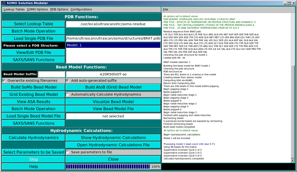SOMO Program:

These functions control the execution of the SOMO program, whose progress is recorded in the right-side main window (in the picture above, a snapshot of the messages during the model building phase of the 8RAT.pdb structure is shown). They are divided in three subpanels controlling operations that deal with the primary PDB file (PDB Functions:), operations relating the generation of bead models (Bead Model Functions:), and the computation of the hydrodynamic parameters (Hydrodynamic Calculations:).

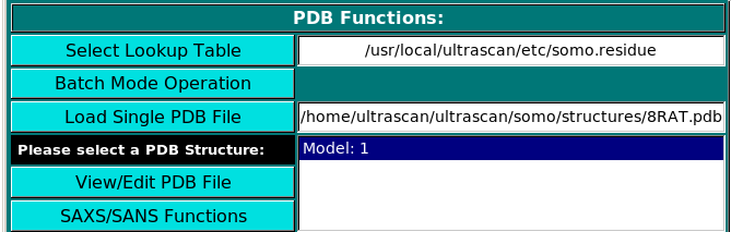PDB Functions:
On launching, US-SOMO will automatically load the last used lookup table (default: somo.residue), where all the informations needed to convert the residues present in atomic structures into beads are stored. To select a different lookup table, click on Select Lookup Table. You can create multiple lookup tables for different conditions. The lookup table needs to contain all atoms and residues present in the (macro)molecule to be loaded in the next step. By default, SOMO will automatically load the last used *.residue table.
Two alternative options are available to load an atomic structure, such as those derived from NMR or X-ray crystallography data, the new Batch Mode Operation (see here), or the standard Load Single PDB File. Selecting a PBD file will also automatically call the molecular visualization program RasMol (Sayle RA, Milner-White EJ. RasMol: biomolecular graphics for all. Trends Biochem. Sci. 20:374-376, 1995) which will display the structure(s) in a pop-up window. For Linux-based systems, RasMol needs to be installed in

$ULTRASCAN/bin

$ULTRASCAN/bin64

Besides visualizing the structure, the HEADER and TITLE fields of the PDB file will be displayed in the progress window, followed by the residues list. If problems are encountered with the selected PDB file, like the presence of non-coded residues or missing atoms within coded residues, they will be reported in the progress window either as warnings or errors. In the latter case, the program execution will be also halted, waiting for corrective action to be taken. The original PDB file can be viewed and, if necessary, edited by clicking on the "View/Edit PDB File button.
The PDB file can contain multiple models and if so, multiple models will be displayed by RasMol and in the list box. In this case, you can select just a single model, or multiple models by holding the crtl key while clicking on the models' names (crtl-A selects all models). If multiple models are selected, all subsequent operations (except the SAXS/SANS options) are carried out sequentially on the selected models. The SAXS/SANS Functions button will also become active, allowing the SAXS- or SANS-related simulations to be carried out on the selected PDB structure. Presently (March 2010), the SAXS/SANS module is under development. (see here)

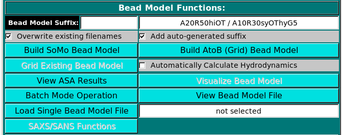Bead Model Functions:
Once one or multiple models are selected, the Build SoMo Bead Model and Build AtoB (Grid) Bead Model buttons will also become active, the last two offering alternative ways of generating a bead model. In the Bead Model suffix field you can enter a tag that will be added to the bead model filename, which is automatically generated from the PDB filename by adding "_1" and the extension ".bead_model". In addition, if the Add auto-generated suffix checkbox is selected, the corresponding field above it is populated with a series of alphanumeric characters specifying the main options chosen. These characters will be also added to the bead model filename, to allow for a quick identification of the options used in its generation. Thus, "A20" stands for a residues' ASA cutoff threshold of 20 A (default), "R50" stands for a bead's ASA re-check cutoff threshold of 50% of its total surface area (default), "hi" signifies hierarchical overlap reduction in all stages (alternatively, "sy" stands for synchronous overlap reduction), and "OT" means that the outward translation option during overlap removal of exposed side-chain beads is active. The "-so" suffix is added if the Build SoMo Bead Model button is then pressed, while the "-a2b" suffix is instead added if the Build AtoB (Grid) Bead Model button is pressed. In this case, the suffix symbols also include "Gn" for the grid resolution, with n the actual value, and "hy" if the atomic-level hydration option is active. Upon loading a PDB file and if the Add auto-generated suffix checkbox is selected, the corresponding field will show the two current strings available for SoMo and AtoB bead models. If any of the options coded in the strings are changed, the field will be automatically updated. The final string will appear once a bead model generation operation is launched. Note that you can keep processing a loaded PDB file after changing any of the various model-building options (see below). If the Overwrite existing filenames checkbox is selected, existing filenames will be overwritten without a warning. Otherwise, a pop up menu will instead appear offering alternative options (see here). The Overwrite existing filenames checkbox is automatically selected for batch mode operations. A third button, Build Grid Bead Model, will operate the Grid routine on a previously generated bead model. This button is not available until a PDB file has been processed with either one of the two bead modeling primary options (see above), or until a previously-generated bead model file has been loaded (see below). If this operation is launched, the "-a2bg" suffix is automatically added to the filename of the new bead model.
Since model building can take some time, depending on the settings and especially for large structures, selecting the Automatic Calculate Hydrodynamics checkbox will allow the direct computation of the hydrodynamic parameters as soon as the model(s) generation has been completed. If this checkbox is not selected (default option), at the end of the model building phase the progress bar will be at 100% and the bead model(s) can be visualized with RasMol by clicking on Visualize Bead Model (recommended, comparing the original structure with the bead model could reveal previously unforeseen problems). The results of the accessible surface area (ASA) computations (see below) can also be visualized in a pop-up window by clicking on the View ASA Results button; this file also includes the computation of the radius of gyration (R_g) directly from the atomic coordinates of the structure. A just-generated or previously-generated bead model file can also be opened inside a text editor by pressing the View Bead Model File button.

Alternatively, you can load one or multiple previously-generated bead model by clicking on either the Batch Mode Operation (see here) or the Load Bead Model File buttons from the menu. In these cases, and if the model(s) was (were) generated/saved in the SOMO format, the various settings/parameters used in model generation will be displayed in the right-side main window. Note that you can decrease the number of beads used, and thus the resolution of the model, by applying a grid procedure on a previously-generated bead model with the Build Grid Bead Model option (see above). This could be useful when large structures are analyzed, although using the improved AtoB routine on the original PDB file while increasing the grid size (Build Grid Bead Model) seems to produce much better results. The SAXS/SANS Functions button present in this subpanel will allow to perform SAXS-or SANS-related simulations directly on the currently loaded bead model. (see here)

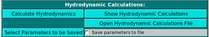Hydrodynamic Calculations:
The hydrodynamic parameters can then be determined by clicking on Calculate Hydrodynamics. A partial list of parameters can be seen in a pop-up window as soon as the calculations are completed by clicking on Show Hydrodynamic Calculations. The pop-up window will also list the solvent type, temperature and its associated density and viscosity, as set in the Hydrodynamic Calculations options module. A full list of all the parameters is also available as a text file, which can be opened from the results' pop-up window. Such a list from a previously analyzed model can be opened also from the Open Hydrodynamic Calculations File button.
The new Select Parameters to be Saved button will open a pop-up window (see here) where characterizing/computed parameters can be selected for saving in a comma-separated file for easy import into spreadsheets. Selecting the Save parameters to file checkbox will generate such file, with extension .csv.

The black bar at the bottom of the progress window will instead report the detailed advancement of some of the steps in the various phases, like the current slice and atoms (or beads) involved in the ASA routine, and the iterations in the supermatrix inversion in the hydrodynamic computations. For small structures, these numbers will be barely flashing by in the box, but for large structures they will allow a more in depth monitoring of the various stages.

Operations can be halted at any moment by clicking on the Stop button. To avoid inadvertendly loosing data, the Close button will not immediately close SOMO, but confirmation will be required in a pop-up window.

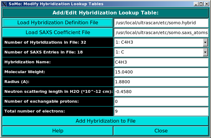
• Add/Edit Hybridization: Use this function to modify the hybridization table. In this file you need to list all hybridizations (as defined in Tsai et al., J. Mol. Biol. 290:253-266, 1999) that will be used for the definitions of all atoms. Each hybridization requires a name, a molecular weight (given by the sum of the mw of the atom being defined plus that of the hydrogen atoms bound to it) and a radius (in Angstrom units). In addition, the neutron scattering length in H₂O, the number of exchangeable protons, and the total number of electrons are entered in this module, because they are needed by the SAXS/SANS simulator module. Load the hybridization file first if one exists, and then the SAXS Coefficients File. This is required because the hybridization table contains also the atom identifiers linking each atom type to its X-ray scattering coefficients. The use of this module is described in this help file.
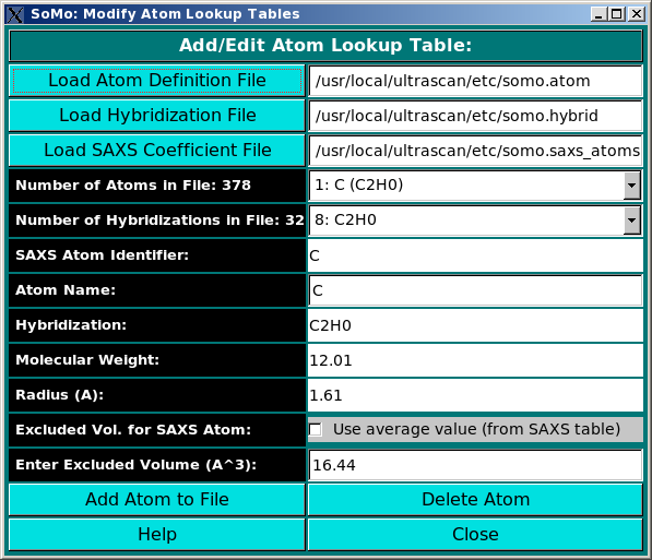
• Add/Edit Atom: Use this function to modify the atom table. In this file the atomic groups present in PDB files are defined, together with their parameters (molecular weight and radius) loaded from the hybridization table. In addition, for SAXS simulation this table is also linked to the SAXS coefficients table, and the excluded volume for each atomic group can be defined in alternative to that of the bare non-hydrogen atom taken from the SAXS coefficient table. The use of this module is described in this help file.
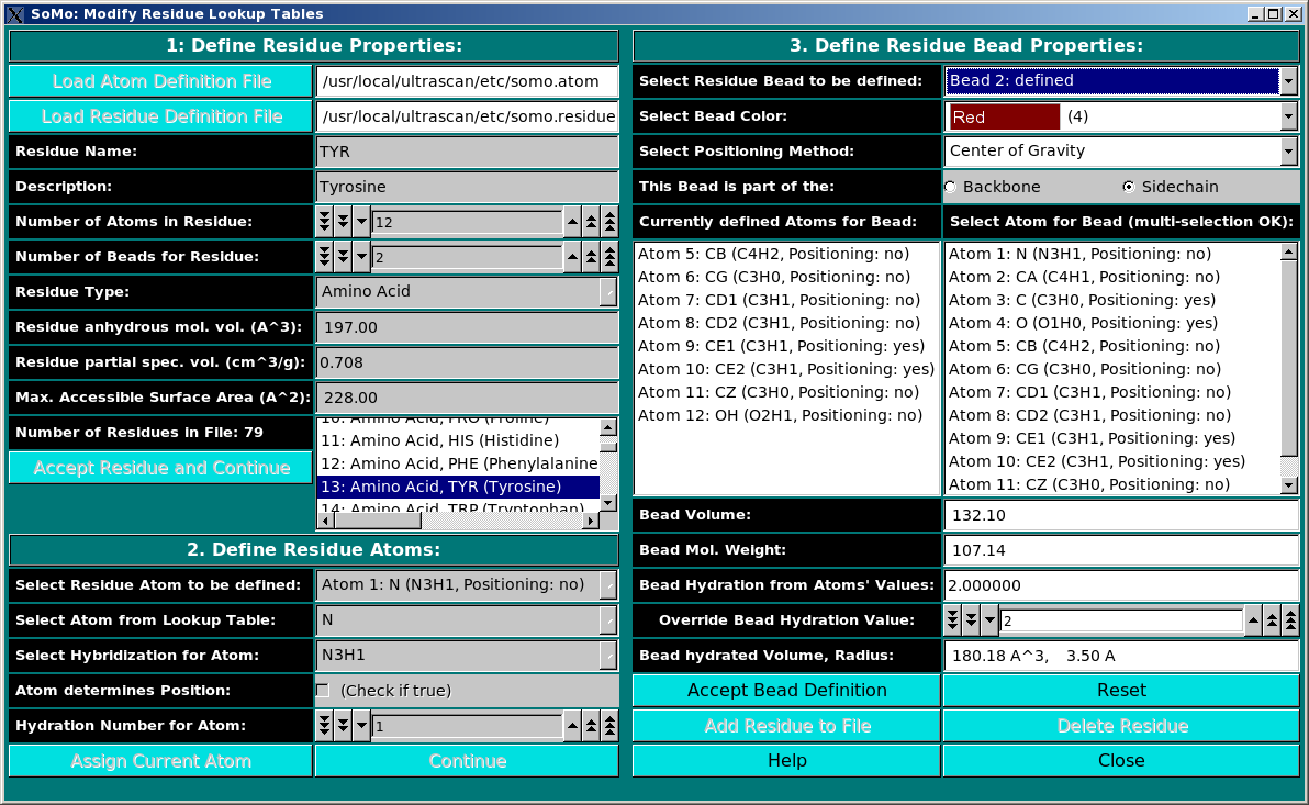
• Add/Edit Residue: Use this function to modify the residue table. This module is used to define all residues that can be found in PDB files. In this module, you can also define the rules which are used to convert them into beads. You can add new residues or modify the properties of the existing ones. The use of this module is described in this help file.
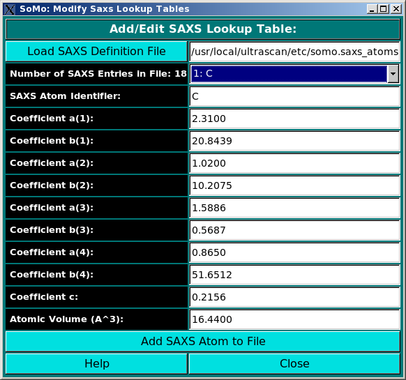
• Add/Edit Saxs Coefficients: Use this function to modify the SAXS coefficients table. In this module, you can add/edit the atomic SAXS coefficients that will be used in the SAXS curve simulator. For each atom, the scattering factor is approximate by a sum of four exponentials requiring eight coefficients and a constant. The values in the somo.saxs_atoms are taken from the International Tables of Crystallography, but can be edited at will. The use of this module is described in this help file.

$ULTRASCAN/etc/somo.config

$HOME/ultrascan/etc/somo.config

• ASA Calculation: Use this function to modify the options for the accessible surface area calculation, which can be done with two alternative methods, SurfRace (Tsodikov OV, Record MT Jr, Sergeev YV. Novel computer program for fast exact calculation of accessible and molecular surface areas and average surface curvature. J. Comput. Chem. 23:600-609, 2002) or ASAB1 (based on Lee B, Richard FM. The interpretation of protein structures: estimation of static accessibility. J. Mol. Biol. 55:379-400, 1971). The second method is also employed for optionally re-checking the accessibility of the beads in the final model. A detailed description of this module can be found here.
• SoMo Overlap Reduction: This module allows you to change the options and handle the various issues related to bead overlap elimination in the SoMo direct correspondence method. A detailed description of this module can be found here.
• AtoB (Grid) Overlap Reduction: This module allows you to change the options and handle the various issues related to bead overlap elimination in the AtoB (Grid) method. A detailed description of this module can be found here.
• Hydrodynamic Calculations: This module allows you to change the options for calculating the hydrodynamic parameters of the bead models. A detailed description of this module can be found here.
• Miscellaneous Options: This module allows you to either automatically compute from the composition or manually enter the partial specific volume of your molecule, and to define the volume used for the hydration water molecules (water of hydration has different properties than "bulk" water). Another option controls the disabling of the peptide bond rule used by the SoMo method to place the main-chain beads. In addition, this module contains the "average" parameters used by the Automatic Bead Builder to generate a single bead for non-coded residues (see here). A detailed description of this module can be found here.
• Bead Model Output: This module allows you to control the options for saving the model(s) in a file (or files). A detailed description of this module can be found here.
• Grid Functions (AtoB): This module allows you to change the options to be used during the bead model generation with the grid function (based on the original program AtoB; Byron O. Construction of hydrodynamic bead models from high-resolution X-ray crystallographic or nuclear magnetic resonance data. Biophys. J. 72:408-415, 1997). The Grid module accepts as input either PDB files or previously-generated bead models. A detailed description of this module can be found here.
• SAXS/SANS Functions: This module will control the setting of the SAXS/SANS curve and P(r) vs. r generator that is currently under development. A detailed description of this module can be found here.

From this pull-down menu, you can access two panels controlling the options for parsing the PDB file and for the model(s) visualization by RasMol.

• Parsing: This module allows you to change the options to be used during the parsing of a PDB file, like how to deal with solvent molecules, explicit hydrogen atoms, alternate conformations, and with missing atoms/residues. A detailed description of this module can be found here. (Remark: some of the options listed are not presently active).
• Visualization: This module allows you to select alternative visualization modes used by RasMol. A detailed description of this module can be found here. (Remark: some of the options listed are not presently active).

• Load Configuration: This button allows you to retrieve a particular set of options previously saved in a user-specified configuration file (see below).
• Save Current Configuration: This button allows you to save the currently selected options for all modules in a user-specified configuration file different from the standard one in which all current parameters are saved when exiting from the program.
• Reset to Default Options: Click on this button to reset all options to default values. The defaults values are stored in a file (somo.defaults), but are also hard-coded in the program. If the somo.defaults file is either missing or doesn't have the right format, US-SOMO will automatically use the hard-coded default values. When exiting just after clicking on this button will reset the standard configuration file as well to default options.
• Advanced Configuration: Clicking on this button will open a pop-up panel allowing the settings of various additional options.