Manual

Finite Element Whole Boundary Fitting Data Analysis:

The Finite Element Whole Boundary Fitting method is based on the numerical solution of the Lamm equation, which is achieved through discretization of the two major variables, radius and scan time, into finite elements. As such, it is possible to accurately model not only the boundary, but also the boundary conditions, such as meniscus and cell bottom. The main purpose of using the Finite Element method is for the modeling of well-defined homogeneous or paucidisperse solutions. This includes single and dual-component systems, simple self-associating systems and isomerizing systems. Modeling with the Finite Element method will result in both s and D, which can be used to calculate f and either molecular weight or the partial specific volume, provided one or the other is known a priori.

Fitting experimental data to a model involves a nonlinear least squares minimization algorithm. This finite element fitting module utilizes the DuD algorithm (Doesn't use Derivatives). Rather than calculating a Jacobian matrix using numerical or analytical derivatives, this method makes a tangent plane approximation to the gradient. It avoids the computationally costly calculation of derivatives. The disadvantage is that it generally requires additional iterations due to the reduced accuracy of the gradient.

You start the Finite Element data analysis by clicking on " Finite Element" in the Velocity sub-menu of the main menu. The main Finite Element Data analysis window will appear.

The first step in the analysis requires that you load an UltraScan dataset that has previously been edited with the UltraScan editing module. UltraScan sedimentation velocity datasets always have the suffix ".us.v". Click on the Load Dataset button in the left upper corner of the control panel. Simply select the desired run from the selection of available runs in the dataset loading dialog. Once loaded, the first available dataset of the selected run will be displayed in the data window on the lower right panel. To start the analysis, a model has to be defined. Click on Create a new Model to define a model. To assist you in defining the proper model it is strongly recommended to analyze the data first by the van Holde - Weischet analysis method. This method will allow you to identify very accurately the presence of multiple components and provide you with reasonable starting guesses for your model. After defining the model, you can start the fitting process by clicking on the button Fitting Control. After fitting is complete, the analysis will be shown in the main window, with the first five residuals shown in the analysis window, and the first five scans overlayed in red with the finite element solution. The fitting control window will indicate the final variance of the last iteration. Next, you can print out the residuals and overlayed data by clicking on the Print Data button, export the result files (Save Data, see File Format Information), or view the Analysis Result Report.

Analysis Functions:

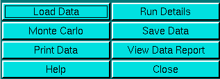
Click on these buttons to control the time derivative analysis. Load Data: Load edited data sets (with the *.us.v suffix). A file dialogue will allow you to select a previously edited and saved velocity experiment. If the data was edited with a previous version of UltraScan, an error message will be displayed. Run Details: View the diagnostic details for a particular run. Monte Carlo: Perform Finite Element Monte Carlo statistics on the analyzed data. Due to the high computational needs of this function, this feature should only be used with the Beowulf/SMP versions of UltraScan. This feature is disabled until a converged fit has been obtained or loaded with Load Fit. Save Data: Write out a copy of all results to an ASCII formatted data file suitable for import into a spreadsheet plotting program. See "File Structures and Formats" for details. Note: These files are overwritten each time this button is clicked. Only the last version of the analysis will be saved! Print Data: Load the printer control panel for printing of plot graphics View Data Report: See the data report for the last analysis setting. Note: This file is re-written each time it is accessed. Only the current analysis result is available. Click here for a sample of a finite element data report Help: This help file Close: Close the Finite Element analysis window.

Run Information:

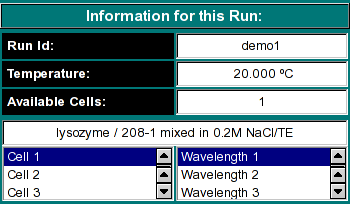
Run ID: The name of the run given during editing Temperature: The average temperature calculated from the entire run Available Cells: The numbers the cells that contain analyzable data Clicking on a cell and wavelength selection will bring up the cell contents description for that cell and wavelength. Scroll through this list to bring up information for cells > 3. If there is no data available for the selected cell, the program will list "No Data available". Selecting a cell/wavelength combination will automatically bring up the corresponding dataset and present the raw data in the lower plot window.

Experimental Parameters:

Here you can enter the corrections for density and viscosity of your buffer. When you change the information in these fields, the program will automatically update the analysis to correct the S-value according to the specified buffer conditions. If you change the settings for density and viscosity after you finished a calculation, be sure to click on the Update for 20oC,W button in the Model Control window to make sure that all parameters are recalculated for the updated buffer settings. Density: Click to calculate the density based on the composition of your buffer. Viscosity: Click to calculate the viscosity based on the composition of your buffer.

Analysis Controls:

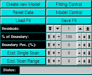
Create new Model: This button allows you to create a new model to be fitted to your data with the finite element analysis Reset Data - use this button to reset the default settings for the analysis. Load Fit: With this function you can recall a previously saved fit (saved with "Save Fit" - see below). It will recall the exact memory state when the fit was saved, including vbar, density and viscosity settings, residuals, raw data and data details. The only requirement is that the file containing the edited data on which the fit is based is available in the "Results Directory" set in the configuration. Fitting Control: This button will recall the fitting control panel. Before pressing this button, a valid model has to be defined. Model Control: This button will recall the model control panel. Before pressing this button, a valid model has to be defined. Save Fit: Use this button to save a converged fit (either for later review or for later Monte Carlo Analysis). The routine will save all pertinent data including the fitted data, the residuals, the parameter values, the model, the hydrodynamic settings (vbar, density, viscosity), data range and excluded scans. Residuals: Once the fitting process has completed, this counter allows you to display the residuals of the fit in groups of 5 scans. Use the counters to select different groups of residuals. The single arrow will move in single steps (5 scans at a time), while the double arrow will advance the groups by 10 with each click (jumps 50 scans). is feature to smooth the experimental data. % of Boundary: This setting allows you to select only a portion of the boundary to be fitted to a finite element solution. Boundary Position (%): Use this counter to move the selected boundary portion up and down between the baseline absorbance and the plateau absorbance. Exlude Single Scan: When setting this counter to a non-zero value, the respective scan will be highlighted in red. Clicking on "Excl. Single Scan" while a scan is highlighted in red will delete this scan from the analysis. Deleting scans from the analysis is irreversible and can only be reset by clicking on the "Reset" button or by reloading the data. Exclude Scan Range: Same as "Exclude Single Scan", except for multiple scans. To use this feature, select first the start scan of the range by using "Exclude Single Scan", then complete the scan range by using "Exclude Scan Range". To be excluded scans are highlighted in red and will be deleted from the dataset when clicking on "Exclude Scan Range". Status: The status bar is reserved for the Beowulf/SMP version of UltraScan to monitor the progress of the Monte Carlo fitting statistics and is without effect for all other UltraScan releases.