Manual

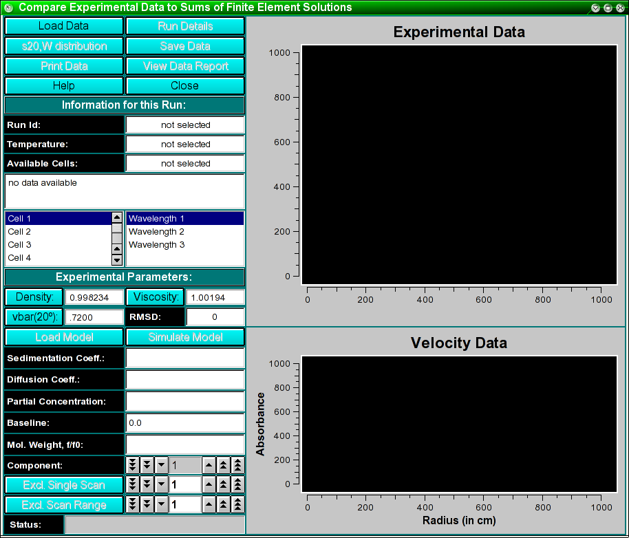
Compare Experimental Data to Sums of Finite Element Solutions

This module is used to import, display and export finite element solutions fitted to velocity experiments by various methods. The program can import models from finite element nonlinear fitting sessions, from 2-dimensional spectrum analysis fits, from genetic algorithm fits, and from C(s) fits. The program will then compare the fitted model to the experimental data and display residual plots, sedimentation and diffusion coefficient distributions, as well as molecular weight distributions. The models can also be displayed as a 3-dimensional plot showing the partial concentrations mapped onto a 2 dimensional grid of any two of the following parameters: s, D, f, f/f0 and MW. Residual plots including deconvoluted time- and radial invariant noise plots can also be displayed. Finally, the results can be saved for inclusion into a velocity result report.

The viewer is started by clicking on the "Finite Element Model Viewer" entry in the Velocity sub-menu of the main menu, which will load the viewer.

Process:

1. Load experimental Data: First, you need to load experimental velocity data. Click on "Load Data" to select an edited velocity dataset from the disk. This dataset should have been fitted by one of the finite element-based analysis methods.

2. Load a Simulation Model: When saving fits prepared in the finite element nonlinear fitting method, the 2-dimensional spectrum analysis, the genetic algorithm mehtod, or the C(s) method, a model file called <run-id>-[fe,sa2d,ga,cofs].model.<cell-number><wavelength-number> will be saved that can then be imported into this viewer module. To load a model, simply click on "Load Model". Once the model is loaded, you can also review the model by clicking on the component counter to display the parameters for each model. The fits can be adjusted on the fly to correct for vbar, density and viscosity by entering the appropriate information. The default setting is for a vbar of 0.72 ccm/g and the viscosity and density of water.

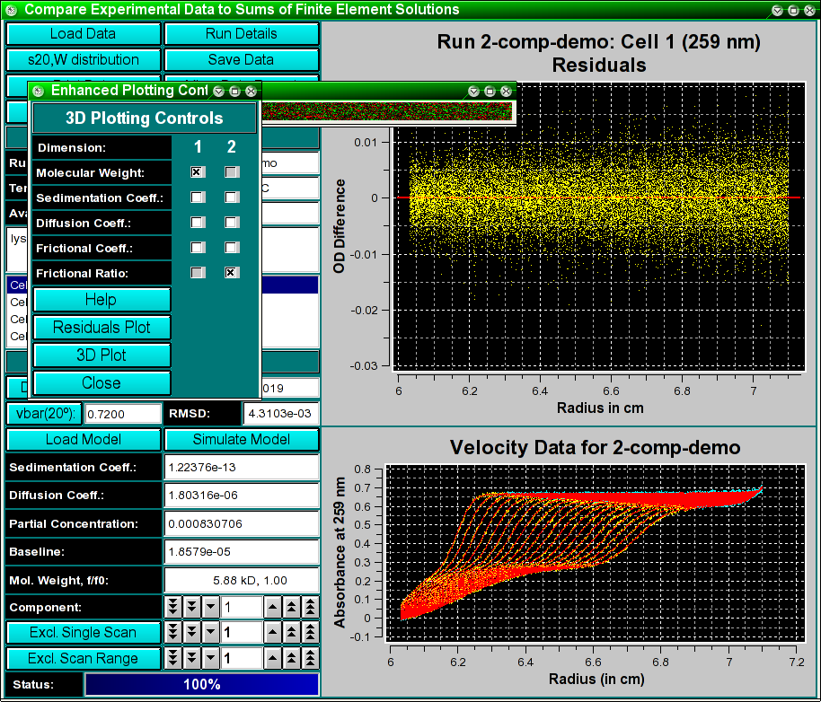
3. Simulate the Model: Next, you need to simulate the loaded model with a finite element solution by clicking on "Simulate Model". After simulation, an RMSD will be calculated, and you will be able to save the fit, review the data plots and residuals. Simulation will allow you to display the distributions of sedimentation and diffusion coefficients, molecular weights, residuals plots and 3-dimensional plots of the loaded model.

4. Save Results After simulation, you will be presented with various dialogs that allow you to plot the results and save them to disk.

Functions:

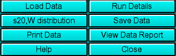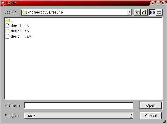
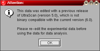
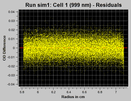
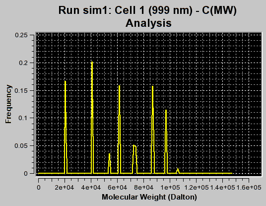
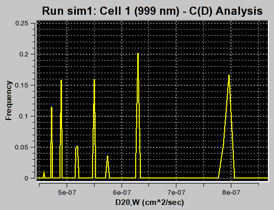
	Load Data: Load edited data sets (with the *.us suffix). A file dialogue will allow you to select a previously edited and saved velocity experiment. If the data was edited with an older version of UltraScan than the current, an error message will be displayed. Run Details: View the diagnostic details for a particular run. s20,W Distribution: This button is a multi-function button that allows you to cycle through four different representations of the data analysis. All representations are shown in the analysis plot section of the module. 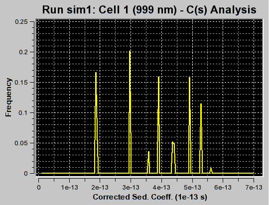The first representation is the residuals pattern, which is shown by default. To change the representation, click on the "C(s) Distribution" button to see the C(s) Distribution. After clicking, you will notice that the button has obtained a different label ("C(MW) Distribution"). The next time you click on it, the program will show the Molecular Weight Distribution obtained after transforming the C(s) distribution to a molecular weight distribution based on the f/f0 and vbar values shown in the Experimental Parameter section. The last representation is the C(D) Distribution, which will show the s-value transformation to a diffusion coefficient distribution based on the f/f0 and vbar values. Save Data: Write out a copy of all results to an ASCII formatted data file suitable for import into a spreadsheet plotting program. Also save the plot images for a report. Note: These files are overwritten each time this button is clicked. Only the last version of the analysis will be saved! Print Data: Load the printer control panel for printing of plot graphics View Data Report: See the data report for the last analysis setting. Note: This file is re-written each time it is accessed. Only the current analysis result is available. Help: This help file Close: Close the viewer window.
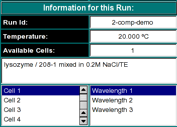	This window will allow you to select the appropriate cell and wavelength from your velocity run.
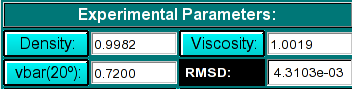	Experimental Parameters Here you can enter the desired vbar, density and viscosity. If the dataset is loaded from the database, these fields are initialized automatically, but can be overridden by the user. The RMSD (residual mean square deviation) is displayed once the model is simulated. It is a measure of the goodness of fit. The RMSD should match the noise level in the data.
	Use these buttons to load the fitted model files and to initiate the simulation of the data.
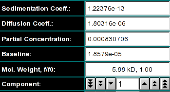	Model Control Here you can display the parameters for each component in the model. Shown are the molecular weight, the sedimentation- and diffusion coefficients, the partial concentration and the baseline of the model. You can select each component of the model, if multiple components are in the model.
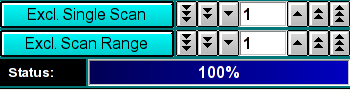	Use this dialog to exclude single scans or scan ranges from the dataset. The status bar indicate the progress in the simulation calculation.
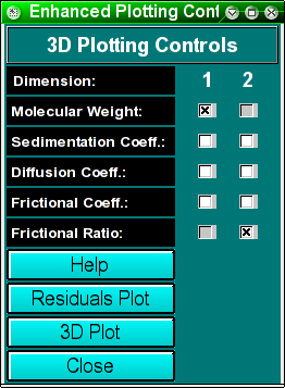	This dialog allows you to control the display of the 3-dimensional plot. You can also request that residual plots be created, as well as display the time invariant and radially invariant noise contributions to your dataset.