Manual

Global Nonlinear Least-Squares Equilibrium Analysis:

Part 6: Fitting Information

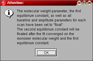
After initializing the parameters for the fit, you should either manually select parameters to be floated by selecting the "Float" checkbox for each parameter you want to be floated, or click on the "Float Parameters" button, which will automatically set all applicable parameters to be floated. A message window will pop up to inform you which parameters have been set to be floated. After clicking on "Float Parameters", the "Check Scans for Fit" button will be activated, and can be used to perform a test, which will confirm that the fit is properly initialized.

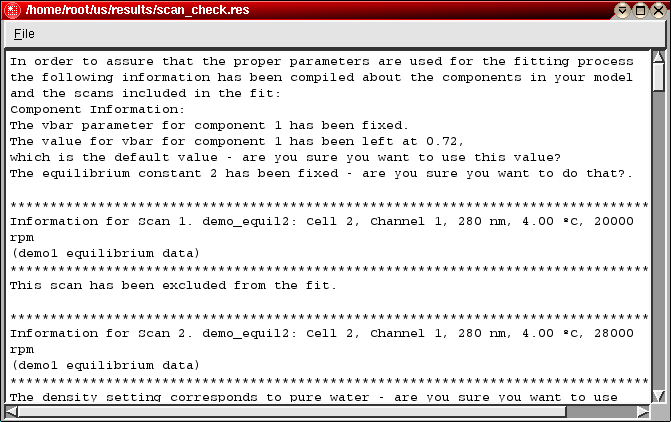
In this test, the following properties will be checked to...

Indicate if the molecular weight or the partial specific volume for a given parameters is floated
Enough scans for a global fit are included (2 minimum are required for a global fit)
make sure that appropriate parameters are floated
Indicate if the partial specific volume has been adjusted or left at the default value of 0.72 ccm/g
Indicate if the buffer density corresponds to the density of pure water
For each scan, indicate if the scan is included or excluded from the fit

Once the test has completed, an information window will be opened which will display the test results. The test results can also be printed, and will be saved to a file called "scan_check.res", which will be saved in your results directory, as configured with the configuration module.

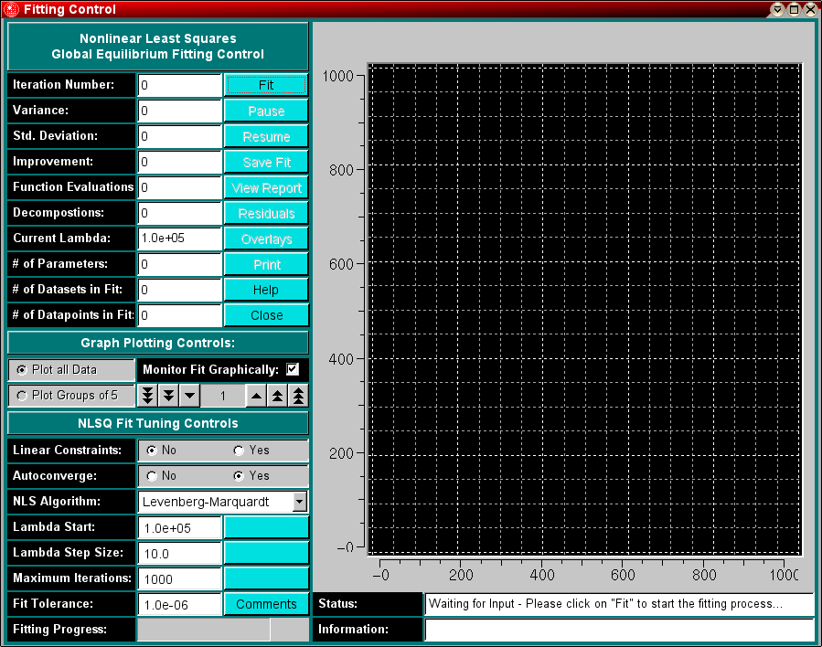
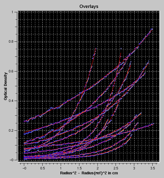
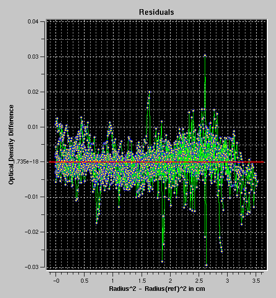
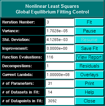
After reviewing the test results, you can proceed to the fitting session by clicking on the "Fitting Control" button, which is now activated. This will invoke the fitting control window. Clicking on the "Fit" button in the fitting control window will start the nonlinear least squares fitting process. Details of this process are explained elsewhere. After fitting has completed, the overlays or residuals will be displayed in the plot window and the result file can be displayed or printed out, by clicking on "View Report" in the fitting control window.

The data analysis report consists out of two sections:

Global Parameter Section:

In the global parameter section, the global run parameters and fitting results will be displayed. Below is an example:

******************************************************************************************
*                              Global Equilibrium Analysis                               *
******************************************************************************************

Data Report for Project "SampleFit"
Fitted Model: Monomer-Dimer Equilibrium

Parameters for this model:

Molecular Weight for component 1: 2.245e+04 dalton (fitted)
Partial Specific Volume for component 1 (at 20C): 7.260e-01 ccm/g (fixed)
Association (Dissociation) Constant 1: 2.073e+10 (4.825e-11)
(fitted)

Global Fitting Statistics:

Variance:                     2.5031e-05
Standard Deviation:           5.0031e-03
Number of floated Parameters: 54
Number of Datasets:           26
Number of Datapoints:         8041
Number of Degrees of Freedom: 7987
Number of Runs:               1340 (31.398 %, corrected)
Expected Number of Runs:      2134 (corrected)
Run Variance:                 1.067e+03 (corrected)

According to these statistical tests, this model is an acceptable candidate for the experimental data.
This fit can be used for a Monte Carlo Analysis with reservations.

The analysis results include a qualitative test of the fitting statistics. "Runs" are a measure for the presence of systematic noise. The presence of systematic noise may indicate that the model is inappropriate for the fit. Models with a large percentage of runs (35 % or better) and a low variance are considered better fits than models with a higher variance and a lower percentage of runs. According to the number of runs in the fit, recommendations are provided concerning the appropriateness of analyzing the model and data with the Monte Carlo Analysis, which can provide reliable statistics for the fit.

Local Parameter Section:
For each scan, individual fitting results and statistics are shown. Excluded scans are indicated. Besides the static parameters for each scan, amplitude, baseline, buoyancy, extinction coefficients and density settings are shown. Integrals corresponding to the relative concentration of the component(s) in the sample are calculated. These integrals are based on the area under the modelled curve between the meniscus (as defined in the editing of the equilibrium run) and the bottom of the cell (as defined by the centerpiece geometry and the rotor stretching, which is calculated based on the rotor selection used in the editing program). Individual fitting statistics are also shown:
```
Detailed Information for fitted Scans:
                                                                                                                                                                             
******************************************************************************************
Information for Scan 1. litai1: Cell 1, Channel 1, 230 nm, 20.00 ºC, 25000 rpm
(wt HSBP1)

Baseline: -7.654e-03 OD (fitted)

Information for component 1:
Amplitude of component 1: -5.293e+00 OD (fitted)
Integral of monomer from Meniscus (6.74700 cm) to bottom (7.20006 cm): 1.209e+00 OD
Integral of multimer 2 from Meniscus (6.74700 cm) to bottom (7.20006 cm): 6.484e+00 OD
Extinction Coefficient for component 1: 5.250e+04
Partial Specific Volume for component 1 (at 20.0C): 0.7260
Buoyancy (20C, H2O):    2.664e-01
Buoyancy, absolute:      2.664e-01
Density Setting:         1.010e+00 g/ccm
Density, absolute:       1.010e+00 g/ccm
Pathlength:              1.200e+00 cm

Fitting Statistics for this Scan:
Raw Point Density:       1.849e-03
Number of Runs:          62 (34.633 %, corrected)
Expected Number of Runs: 87 (corrected)
Run Variance:            4.171e+01 (corrected)
```
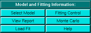
Should you decide to perform a Monte Carlo analysis on your fit, you will need to first save the fit by clicking on the "Save Fit" button in the fitting control window. Next, you can click on the "Monte Carlo" button in the Model and Fitting Information section of the Global Equilibrium Fitting Window. More information on the Monte Carlo analysis is available here, a Monte Carlo tutorial is also available.

Previous: Parameter Controls Fitting Information Next: Model-Specific Information
www contact: Borries Demeler
This document is part of the UltraScan Software Documentation distribution.
Copyright © notice
The latest version of this document can always be found at:
Last modified on January 12, 2003.