
|
|
Manual |
This document discusses how to use the Nonlinear Least Squares fitting routine included with UltraScan. Global equilibrium data analysis, finite element fitting and global extinction profile fitters all use this routine, and share this interface.
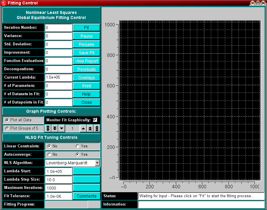
Depending on which routine invoked the fitter, the interface will have a different label:
| Finite Element (AD): |  |
| Global Equilibrium: |  |
| Global Wavelength Fitter: |  |
Explanation of Fields and Buttons:
|
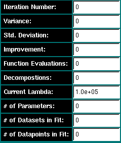
Iteration Number: | The program will keep track on each nonlinear least squares iteration and list the current iteration here. The program will abort if the maximum number of iterations has been reached. The maximum number of iterations can be adjusted in the "NLSQ Fit Tuning Controls" (see below). |
| Variance: | This field indicates the variance from the current iteration. | |
| Std. Deviation | This field indicates the standard deviation (square-root of the variance) for the current iteration. | |
| Improvement: | This field indicates the variance improvement between the current and previous iteration. | |
| Function Evaluations | Lists the number of times the model/objective function has been evaluated. | |
| Decompositions: | The number of Cholesky decompositions of the information matrix. | |
| Current Lambda | The value of the current step size/lambda. What lambda represents depends on the nonlinear least squares fitting algorithm that was chosen. | |
| # of Parameters | Number of parameters floated in the fit. | |
| # of Datasets in Fit | The number of scans or datasets included in the global fit | |
| # of Datapoints in Fit | The sum of all datapoints in the fit. The number of degrees of freedom in the fit can be calculated by subtracting the number of parameters from the number of datapoints in the fit. | |
|
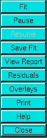
Fit | Start fitting and look for a global minimum. This button will be disabled during a fit in progress. |
| Pause | Pause an ongoing fit - this button will be disabled while no fit is in progress. | |
| Resume | Resume a paused fit. This button is disabled at all times, except when a fit is paused. | |
| Save Fit | Save a memory tate opy of the current fit. The fit can be recalled later and continued at the same point where it was left off. Make sure the fit has converged before saving it. Do not save a paused fit. | |
| View Report | View the data analysis report. Formats differ depending on what model and experiment is fitted. | |
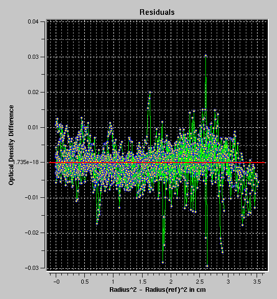
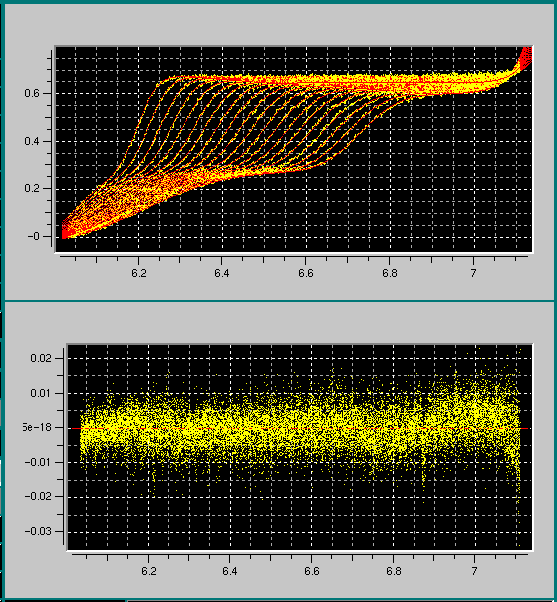
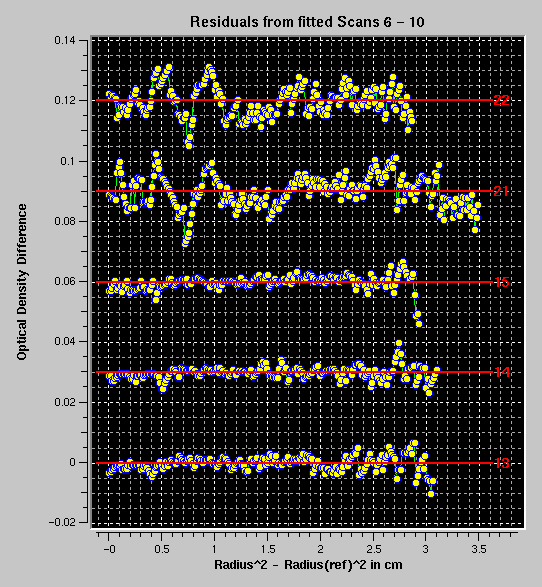
| Residuals | After the fit has converged, you can display residuals of the fit by clicking on this button. Some modules show both residuals and overlay plots simultaneously (for example, the finite element fitter), and this feature is disabled. | |
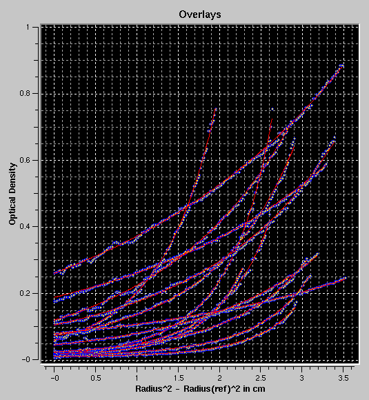
| Overlays | After the fit has converged, you can display overlays of the fit by clicking on this button. Some modules show both residuals and overlay plots simultaneously (for example, the finite element fitter), and this feature is disabled. | |
| Print the plot currently in the plot window. Use the Printer Control module to select print properties, and also which plot to print in case more than one plotwindow are available (for example, in the finite element fitter, which shows the residuals and overlays simultaneously. | ||
| Help | Open this help window | |
| close | Close this program and exit | |
|
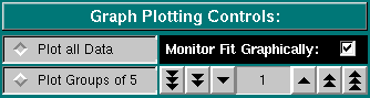
Plot all Data | Selecting this checkbox will plot all data combined on the same graph. While all nonlinear least squares applications provide residuals and overlay plots, this selection also affects other plots that may be available depending on the type of data and selected fitting method. |
| Monitor Fit Graphically | When checked, this allows you to watch the progress of the fit graphically, either as residuals or as overlays. If unchecked, the plot is only updated once it is converged. | |
| Plot Groups of 5 | Selecting this checkbox will plot data in groups of 5 on the same graph. While all nonlinear least squares applications provide residuals and overlay plots, this selection also affects other plots that may be available depending on the type of data and selected fitting method. By clicking on the counter you can select different groups of 5. | |
|
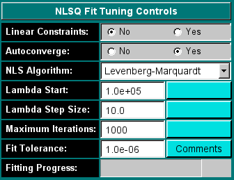
Linear Constraints | (not implemented yet) |
| Autoconverge | When enabled, this feature automatically switches between Levenberg-Marquardt and the Quasi-Newton method algorithms to improve convergence. Particularly for large fits with many parameters fits can get stuck in local minima. A local minimum in one algorithm is often not a local minimum in another, so by trying multiple algorithms, it is often possible to improve the fit. When turned off, the user can accomplish the same capability by switching manually between multiple algorithms until all attempted algorithms converge within one iteration. | |
| NLS Algorithm: |
Select the nonlinear least squares fitting algorithm. Choices are:
|
|
| Lambda Start: | Starting value of Lambda. Set to a large number (1x10⁷ if initial iterations collapse. | |
| Lambda Step Size: | The stepsize adjustment made to lambda during each iteration. | |
| Maximum Iterations: | If this number is reached, the fitting process aborts. | |
| Fit Tolerance: | The fit is considered converged when this value is reached, or when the variance cannot be decreased any further than this value. | |
| Fitting Progress | Attempts to guess the finish of the fitting process by estimating the number of iterations required to reach convergence. The estimate is based on the halving of the variance between successive iterations. | |
| Comments | Click here to enter comments for your fit. These comments will be included in the html reports that can be generated for various experiments. | |
| Other fields | Blank fields are placeholders for supplemental plots available in selected fitting methods. These are discussed elsewhere. |
This document is part of the UltraScan Software Documentation
distribution.
Copyright © notice.
The latest version of this document can always be found at:
Last modified on January 12, 2003.